Artificial Neural Networks have gained attention during the recent years, driven by advances in deep learning. But what is an Artificial Neural Network and what is it made of?

Meet the perceptron.

In this article we’ll have a quick look at artificial neural networks in general, then we examine a single neuron, and finally (this is the coding part) we take the most basic version of an artificial neuron, the perceptron, and make it classify points on a plane.

But first, let me introduce the topic.

Artificial neural networks as a model of the human brain

Have you ever wondered why there are tasks that are dead simple for any human but incredibly difficult for computers? Artificial neural networks (short: ANN’s) were inspired by the central nervous system of humans. Like their biological counterpart, ANN’s are built upon simple signal processing elements that are connected together into a large mesh.

What can neural networks do?

ANN’s have been successfully applied to a number of problem domains:

• Classify data by recognizing patterns. Is this a tree on that picture?
• Detect anomalies or novelties, when test data does not match the usual patterns. Is the truck driver at the risk of falling asleep? Are these seismic events showing normal ground motion or a big earthquake?
• Process signals, for example, by filtering, separating, or compressing.
• Approximate a target function–useful for predictions and forecasting. Will this storm turn into a tornado?

Agreed, this sounds a bit abstract, so let’s look at some real-world applications. Neural networks can -

• identify faces,
• recognize speech,
• read your handwriting (mine perhaps not),
• translate texts,
• play games (typically board games or card games)
• control autonomous vehicles and robots
• and surely a couple more things!

The topology of a neural network

There are many ways of knitting the nodes of a neural network together, and each way results in a more or less complex behavior. Possibly the simplest of all topologies is the feed-forward network. Signals flow in one direction only; there is never any loop in the signal paths.

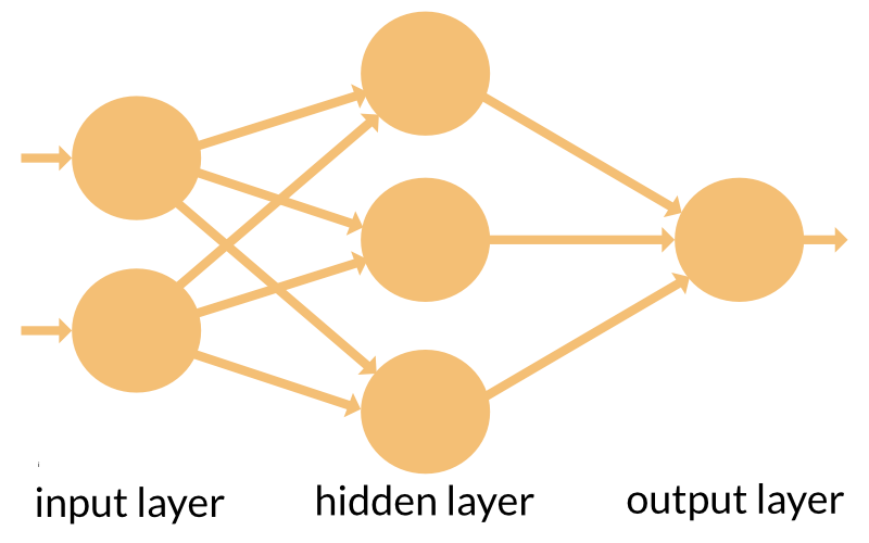
Typically, ANN’s have a layered structure. The input layer picks up the input signals and passes them on to the next layer, the so-called ‘hidden’ layer. (Actually, there may be more than one hidden layer in a neural network.) Last comes the output layer that delivers the result.

Neural networks must learn

Unlike traditional algorithms, neural networks cannot be ‘programmed’ or ‘configured’ to work in the intended way. Just like human brains, they have to learn how to accomplish a task. Roughly speaking, there are three learning strategies:

Supervised learning

The easiest way. Can be used if a (large enough) set of test data with known results exists. Then the learning goes like this: Process one dataset. Compare the output against the known result. Adjust the network and repeat. This is the learning strategy we’ll use here.

Unsupervised learning

Useful if no test data is readily available, and if it is possible to derive some kind of cost function from the desired behavior. The cost function tells the neural network how much it is off the target. The network then can adjust its parameters on the fly while working on the real data.

Reinforced learning

The ‘carrot and stick’ method. Can be used if the neural network generates continuous action. Follow the carrot in front of your nose! If you go the wrong way - ouch. Over time, the network learns to prefer the right kind of action and to avoid the wrong one.

Ok, now we know a bit about the nature of artificial neural networks, but what exactly are they made of? What do we see if we open the cover and peek inside?

Neurons: The building blocks of neural networks

The very basic ingredient of any artificial neural network is the artificial neuron. They are not only named after their biological counterparts but also are modeled after the behavior of the neurons in our brain.

Biology vs technology

Just like a biological neuron has dendrites to receive signals, a cell body to process them, and an axon to send signals out to other neurons, the artificial neuron has a number of input channels, a processing stage, and one output that can fan out to multiple other artificial neurons.

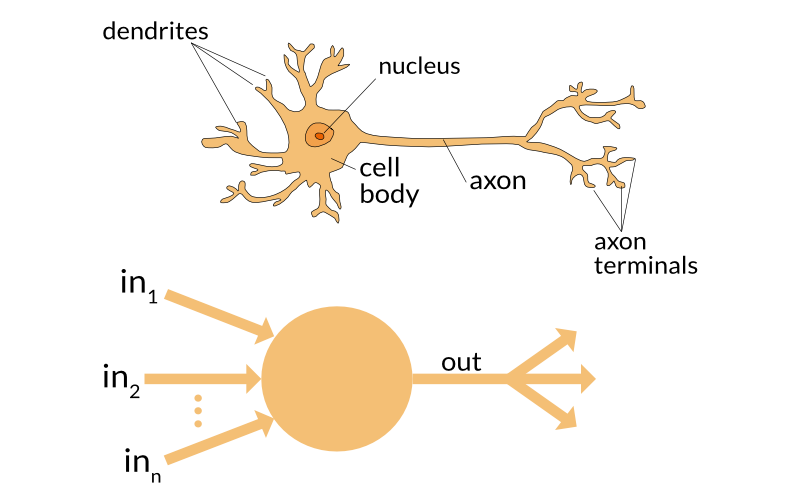
Inside an artificial neuron

1. Each input gets scaled up or down

When a signal comes in, it gets multiplied by a weight value that is assigned to this particular input. That is, if a neuron has three inputs, then it has three weights that can be adjusted individually. During the learning phase, the neural network can adjust the weights based on the error of the last test result.

2. All signals are summed up

In the next step, the modified input signals are summed up to a single value. In this step, an offset is also added to the sum. This offset is called bias. The neural network also adjusts the bias during the learning phase.

This is where the magic happens! At the start, all the neurons have random weights and random biases. After each learning iteration, weights and biases are gradually shifted so that the next result is a bit closer to the desired output. This way, the neural network gradually moves towards a state where the desired patterns are “learned”.

3. Activation

Finally, the result of the neuron’s calculation is turned into an output signal. This is done by feeding the result to an activation function (also called transfer function).

The perceptron

The most basic form of an activation function is a simple binary function that has only two possible results.

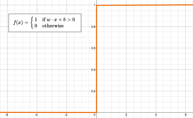
Despite looking so simple, the function has a quite elaborate name: The Heaviside Step function. This function returns 1 if the input is positive or zero, and 0 for any negative input. A neuron whose activation function is a function like this is called a perceptron.

Can we do something useful with a single perceptron?

If you think about it, it looks as if the perceptron consumes a lot of information for very little output - just 0 or 1. How could this ever be useful on its own?

There is indeed a class of problems that a single perceptron can solve. Consider the input vector as the coordinates of a point. For a vector with n elements, this point would live in an n-dimensional space. To make life (and the code below) easier, let’s assume a two-dimensional plane. Like a sheet of paper.

Further consider that we draw a number of random points on this plane, and we separate them into two sets by drawing a straight line across the paper:

This line divides the points into two sets, one above and one below the line. (The two sets are then called linearly separable.)

A single perceptron, as bare and simple as it might appear, is able to learn where this line is, and when it finished learning, it can tell whether a given point is above or below that line.

Imagine that: A single perceptron already can learn how to classify points!

Let’s jump right into coding, to see how.

The code: A perceptron for classifying points

1
2
3
4
5
6
7
8
9
10
11
12
13
14
15
16
17
18
19
20
21
22
23
24
25
26
27
28
29
30
31
32
33
34
35
36
37
38
39
40
41
42
43
44
45
46
47
48
49
50
51
52
53
54
55
56
57
58
59
60
61
62
63
64
65
66
67
68
69
70
71
72
73
74
75
76
77
78
79
80
81
82
83
84
85
86
87
88
89
90
91
92
93
94
95
96
97
98
99
100
101
102
103
104
105
106
107
108
109

package main

import (
    "fmt"
    "math/rand"
    "time"
    "github.com/appliedgo/perceptron/draw"
)

type Perceptron struct {
    weights []float32
    bias float32
}

func (p *Perceptron) heaviside(f float32) int32 {
    if f < 0 {
        return 0
    }
    return 1
}

func NewPerceptron(n int32) *Perceptron {
    var i int32
    w := make([]float32, n, n)
    for i = 0; i < n; i++ {
        w[i] = rand.Float32()*2 - 1
    }
    return &Perceptron{
        weights: w,
        bias: rand.Float32()*2 - 1
    }
}

func (p *Perceptron) Process(inputs []int32) int32 {
    sum := p.bias
    for i, input := range inputs {
        sum += float32(input) * p.weights[i]
    }
    return p.heaviside(sum)
}

func (p *Perceptron) Adjust(inputs []int32, delta int32, learningRate float32) {
    for i, input := range inputs {
        p.weights[i] += float32(input) * float32(delta) * learningRate
    }
    p.bias += float32(delta) * learningRate
}

var (
    a, b int32
)

func f(x int32) int32 {
    return a*x + b
}

func isAboveLine(point []int32, f func(int32) int32) int32 {
    x := point[0]
    y := point[1]
    if y > f(x) {
        return 1
    }
    return 0
}

func train(p *Perceptron, iters int, rate float32) {
    for i := 0; i < iters; i++ {
        point := []int32{
            rand.Int31n(201) - 101,
            rand.Int31n(201) - 101,
        }
        actual := p.Process(point)
        expected := isAboveLine(point, f)
        delta := expected - actual
        p.Adjust(point, delta, rate)
    }
}

func verify(p *Perceptron) int32 {
    var correctAnswers int32 = 0
    c := draw.NewCanvas()
    
    for i := 0; i < 100; i++ {
        point := []int32{
            rand.Int31n(201) - 101,
            rand.Int31n(201) - 101,
        }
        result := p.Process(point)
        if result == isAboveLine(point, f) {
            correctAnswer += 1
        }
        c.DrawPoint(point[0], point[1], result == 1)
    }
    c.DrawLinearFunction(a, b)
    c.Save()
    return correctAnswers
}

func main() {
    rand.Seed(time.Now().UnixNano())
    a = rand.Int31n(11) - 6
    b = rand.Int31n(101) - 51
    p := NewPerceptron(2)
    iterations := 1000
    var learningRate float32 = 0.1
    train(p, iterations, learningRate)
    successRate := verify(p)
    fmt.Printf("%d%% of the answers were correct\n", successRate)
}

Exercises

1. Play with the number of training iterations!

   • Will the accuracy increase if you train the perceptron 10,000 times?
   • Try fewer iterations. What happens if you train the perceptron only 100 times? 10times?
   • What happens if you skip the training completely?

2. Change the learning rate to 0.01, 0.2, 0.0001, 0.5, 1,… while keeping the training iterations constant. Do you see the accuracy change?