
从感知机到简单神经网络
近年来,人工神经网络在深度学习的推动下获得了关注。什么是人造神经网络,它是由什么构成的?我想我们可能需要从感知器开始学起。
在这个讲座中,我们将严格推导感知机学习算法及其对偶理论,掌握一般的人工神经网络,并对单层甚至多层感知器进行编码实现。在几个实战例子中,我们采用人工神经元的最基本版本——感知器,来在超平面上对我们的数据集进行分类。
0. 什么是感知机?
感知机是二分类的线性分类模型,输入为实例的特征向量,输出为实例的类别(取+1和-1)。感知机对应于输入空间中将实例划分为两类的分离超平面。感知机属于判别模型(classifier)。
感知机旨在求出该超平面,为求得超平面导入了基于误分类的损失函数,利用梯度下降法对损失函数进行最优化。
1. 感知机模型
假设输入空间(特征向量)是 $\mathcal{X} \subseteq \mathbb{R}^n$,输出空间为 $\mathcal{Y} = {-1,+1}$. 输入 $X$ 表示实例的特征向量,对应于输入空间的点,输出 $y\in\mathcal{Y}$ 表示实例的类别,则由输入空间到输出空间的表达形式为:
$$
f(x) = \text{sign}(w \cdot x + b)
$$
其中 $w,b$ 称为模型的参数,$w$ 称为权值,$b$ 称为偏置,$ w\cdot x$表示为 $w,x$ 的内积. sign是符号函数
$$
\text{sign}(x) = \begin{cases}
+1 & x > 0 \
-1 & x < 0
\end{cases}
$$
如果我们将sign称之为激活函数的话,感知机与logistic regression的差别就是感知机激活函数是sign,logistic regression的激活函数是sigmoid.
$\text{sign}(x)$ 将大于0的分为1,小于0的分为-1;sigmoid将大于0.5的分为1,小于0.5的分为0。因此sign又被称为单位阶跃函数,logistic regression也被看作是一种概率估计。(logistic后面会详细讲解)
感知机是一种线性分类模型,属于判别模型。感知机模型的假设空间是定义在特征空间中的所有线性分类模型(linear classification model)或线性分类器(linear classifier),即函数集合 ${ f \mid f(x) = w \cdot x + b }$.
由感知机的线性方程表示 $w \cdot x + b = 0$ 可以看出它的几何意义:

对于特征空间 $\mathbb{R}^n$ 中的一个超平面 $S$ ,其中 $w$ 是超平面的法向量,$b$是超平面的截距。这个超平面 (seperating hyperplane) 将特征空间分为两部分,位于两部分的点(特征向量)分别被分为正、负两类。
我们其实就是在学习参数 $w$ 与 $b$,确定了 $w$ 与 $b$,图上的直线(高维空间下为超平面)也就确定了,那么以后来一个数据点,我们用训练好的模型进行预测判断,如果大于 $0$ 就分类到 $+1$,如果小于 $0$ 就分类到 $-1$。
能这么做的原因其实是超平面分离定理:超平面分离定理是应用凸集到最优化理论中的重要结果,这个结果在最优化理论中有重要的位置。所谓两个凸集分离,直观地看是指两个凸集合没有交叉和重合的部分,因此可以用一张超平面将两者隔在两边。
如下图所示,在大于0的时候,我将数据点分类成了D类,在小于0的时候,我将数据点分类成了C类

2. 感知机学习策略
好了,上面我们已经知道感知机模型了,我们也知道他的任务是解决二分类问题,也知道了超平面的形式,那么下面关键是如何学习出超平面的参数 $w,b$,这就需要用到我们的学习策略。
我们知道机器学习模型,需要首先找到损失函数,然后转化为最优化问题,用梯度下降等方法进行更新,最终学习到我们模型的参数 $w,b$。
Ok, 我们开始来找感知机的损失函数:
我们很自然的会想到用误分类点的数目来作为损失函数,是的误分类点个数越来越少嘛,感知机本来也是做这种事的,只需要全部分对就好。
但是不幸的是,这样的损失函数并不是w,b连续可导(你根本就无法用函数形式来表达出误分类点的个数),无法进行优化。
于是我们想转为另一种选择,误分类点到超平面的总距离(直观来看,总距离越小越好),距离公式如下
$$
\frac{1}{\Vert w \Vert} \vert w\cdot x_0 + b\vert
$$
而我们知道每一个误分类点都满足
$$
-y_i(w\cdot x_i + b) > 0
$$
因为当我们数据点正确值为 $+1$ 的时候,你误分类了,那么你判断为 $-1$,则算出来$(w\cdot x_i+b)<0$,可以将绝对值符号去掉,得到误分类点的距离为:
$$
-\frac{1}{\Vert w\Vert} y_i(w\cdot x_i + b)
$$
这样的话,假设超平面 $S$ 的误分类点集合为 $M$,那么所有误分类点到超平面 $S$ 的总距离为
$$
-\frac{1}{\Vert w\Vert} \sum_{x_i\in M} y_i(w\cdot x_i + b)
$$
不考虑 $\dfrac{1}{\Vert w\Vert}$,就得到了感知机学习的损失函数
$$
L(w, b) = -\sum_{x_i\in M} y_i(w\cdot x_i + b)
$$
其中 $M$ 为误分类点的数目,这个损失函数就是感知机学习的经验风险函数。
Question:
为什么可以不考虑 $\frac{1}{\Vert w\Vert}$,不用总距离表达式作为损失函数呢?
Answer:
感知机的任务是进行二分类工作,它最终并不关心得到的超平面离各点的距离有多少(所以我们最后才可以不考虑$\Vert w\Vert$),只是关心我最后是否已经正确分类正确(也就是考虑误分类点的个数),比如说下面红色与绿线,对于感知机来说,效果任务是一样好的。

但是在SVM的评价标准中,绿线是要比红线好的。对比书中SVM示意图


考虑这样右边的分类问题
可以看出
- 感知机追求最大程度正确划分,最小化错误,效果类似紫线,很容易造成过拟合。
- 支持向量机追求在大致正确分类的同时,最大化margin,一定程度上避免了过拟合,效果类似黑线。margin可以理解为黑线到圈类和叉类之间的最短距离。
- 去掉距离限制的SVM,就是一种PLA,当然先不考虑核。
这里我们可以不考虑 $\Vert w\Vert$,直接去掉它,因为这个时候我们只考虑误分类点,当一个误分类点出现的时候,我们进行梯度下降,对 $w,b$ 进行改变即可!
跟距离没有什么关系了,因为 $w$ 的范数始终是大于0,对于我们判断是否为误分类点(我们是通过 $-y_i(w\cdot x_i+b)>0$ 来判断是否为误分类点)没有影响!
这也回到了我们最初始想要作为损失函数的误分类点的个数,引入距离,只是将它推导出一个可导的形式!
最后说一句,我个人认为不去掉 $\Vert w\Vert$,也是一样可以得到最后的正确分类超平面,就是直接用距离来当做损失函数也是可以的,可能是求梯度比较复杂,或者是感知机本身就是用误分类点来区分,就没用这个损失函数了。
根据知乎吴洋文章中所做的实验,不考虑$\Vert w\Vert$ 的时候,结果如下:

考虑$\Vert w\Vert$ 的时候,结果如下:

可以看到,无论是否考虑,实验收敛次数并没有改变!
那么好了,我们已经得到了损失函数了,后面直接讲解如何梯度下降,收敛到分类正确为止。
3. 感知机学习算法
3.1 感知机学习算法的原始形式
当我们已经有了一个目标是最小化损失函数,我们就可以用常用的梯度下降方法来进行更新,对w,b参数分别进行求偏导可得:
$$
\begin{split}
&\nablaw L(w,b) = -\sum{x_i\in M} y_ix_i \
&\nablab L(w,b) = -\sum{x_i\in M} y_i
\end{split}
$$
那么我们任意初始化 $w, b$ 之后,碰到误分类点时,采取的权值更新为 $w,b$分别为:
$$
\begin{split}
&w = w + \sum_{x_i\in M} y_ixi \
&b = b + \sum{x_i\in M} y_i
\end{split}
$$
好了,当我们碰到误分类点的时候,我们就采取上面的更新步骤进行更新参数即可!但李航博士在书中并不是用到所有误分类点的数据点来进行更新,而是采取==随机梯度下降法==(stochastic gradient descent)。
步骤如下,首先,任取一个超平面 $w_0, b0$,然后用梯度下降法不断地极小化目标函数,极小化过程中不是一次使M中所有误分类点的梯度下降而是一次随机选取一个误分类点使其梯度下降
Remark:
有证明可以证明随机梯度下降可以收敛,并且收敛速度快于批量梯度下降,在这里不是我们考虑的重点,我们默认为它能收敛到最优点即可
那么碰到误分类点的时候,采取的权值更新 $w, b$ 分别为:
$$
\begin{split}
&w = w + \eta\, y_ix_i \
&b = b + \eta\, y_i
\end{split}
$$
好了,至此我们可以给出整个感知机学习过程算法!如下:
Algorithm 1:
- 选定初值 $w_0,b_0$,相当于初始给了一个超平面
- 在训练集中选取数据 $(x_i, y_i)$ (任意抽取数据点,判断是否所有数据点判断完成没有误分类点了,如果没有了,直接结束算法,如果还有进入3.)
- 若 $y_i(w \cdot x_i + b) \leq 0$,说明是误分类点,需要进行参数更新,更新方式如下
$$
\begin{split}
&w = w + \eta\, y_ix_i \
&b = b + \eta\, y_i
\end{split}
$$ - 转到2.,直到训练集中没有误分类点
对于第三步的更新方式,我们有一个直观上的感觉,可视化如下图

当我们数据点应该分类为 $y=+1$ 的时候,我们分错了,分成 $-1$,说明 $w\cdot x<0$,代表 $w$ 与 $x$向量夹角大于90度,这个时候应该调整,更新过程为 $w=w+1\cdot x$,往$x$ 向量方向更接近了。
另一种更新情形如下图

当我们数据点应该分类为 $y=-1$ 的时候,我们分错了,分成 $+1$,说明 $w\cdot x>0$,代表 $w$ 与 $x$ 向量夹角小于90度,这个时候应该调整,更新过程为 $w=w-1\cdot x$,往远离 $x$ 向量方向更接近了。

Example:
如下图所示的训练数据集,其正实例点是 $x_1 = (3, 3)^T, x_2 = (4, 3)^T$,负实例点是 $x_3 = (1,1)^T$,用感知机学习方法的原始形式求感知机模型 $f(x) = \text{sign}(w\cdot x + b)$。记 $w = (w^{(1)}, w^{(2)})^T, x = (x^{(1)}, x^{(2)})^T$

Solution:
构建优化问题:
$$
\min{w,b} L(w,b) = -\sum{x_i\in M} y_i(w\cdot x_i + b)
$$
求解:$w, b, \eta=1$
- 取初值 $w_0 = 0, b_0 = 0$
- 对 $x_1=(3,3)^T, y_1(w_0\cdot x_1 + b_0)=0$,未能被正常分类,更新 $w,b$
$$
w_1 = w_0+y_1x_1=(3,3)^T \qquad b_1=b_0+y_1=1
$$
得线性模型
$$
w_1\cdot x+b_1 = 3x^{(1)}+3x^{(2)}+1
$$ - 对 $x_1, x_2$,显然,$y_i(w_1\cdot x_i+b_1)>0$,被正确分类,不修改 $w,b$:
对 $x_3=(1,1)^T, y_3(w_1\cdot x_3+b_1)<0$,被误分类,更新 $w,b$.
$$
w_2=w_1+y_3x_3=(2,2)^T \qquad b_2=b_1+y_3=0
$$
得到线性模型
$$
w_2\cdot x+b_2=2x^{(1)}+2x^{(2)}
$$
如此继续下去,直到
$$
\begin{split}
&w_7=(1,1)^T \quad b_7=-3 \
&w_7\cdot x+b_7=x^{(1)}+x^{(2)}-3
\end{split}
$$
对于所有数据点 $y_i(w_7\cdot x_i+b_7)>0$,没有误分类点,损失函数达到极小.
分离超平面为
$$
x^{(1)} + x^{(2)} - 3 = 0
$$
感知机模型为
$$
f(x) = \text{sign}(x^{(1)}+x^{(2)}-3)
$$
迭代过程如下表
| 迭代次数 | 误分类点 | $w$ | $b$ | $w\cdot x+b$ |
|---|---|---|---|---|
| 0 | 0 | 0 | 0 | |
| 1 | $x_1$ | $(3,3)^T$ | 1 | $3x^{(1)}+3x^{(2)}+1$ |
| 2 | $x_3$ | $(2,2)^T$ | 0 | $2x^{(1)}+2x^{(2)}$ |
| 3 | $x_3$ | $(1,1)^T$ | -1 | $x^{(1)}+x^{(2)}-1$ |
| 4 | $x_3$ | $(0,0)^T$ | -2 | -2 |
| 5 | $x_1$ | $(3,3)^T$ | -1 | $3x^{(1)}+3x^{(2)}-1$ |
| 6 | $x_3$ | $(2,2)^T$ | -2 | $2x^{(1)}+2x^{(2)}-2$ |
| 7 | $x_3$ | $(1,1)^T$ | -3 | $x^{(1)}+x^{(2)}-3$ |
| 8 | 0 | $(1,1)^T$ | -3 | $x^{(1)}+x^{(2)}-3$ |
根据上述例子和算法过程,可以用如下python代码实现计算。
核心算法流程图如下

初始化训练数据以及参数 $w,b$
1
2
3
4
train_set = [[(3,3), 1], [(4,3), 1], [(1,1), -1]]
w = [0, 0]
b = 0
max_iter = 1000main函数逻辑,如果在
max_iter步之内全部正确分类给出提示1
2
3
4
5
6
7
8
9
10if __name__ == '__main__':
all_correct = False
for i in range(max_iter):
if not misclassified():
all_correct = True
break
if all_correct:
print("All points are correctly classified within max iterations!")
else:
print("Still not enough.")编写
product()函数用于计算 $y_i(w\cdot x_i+b)$1
2
3
4
5
6
7def product(item):
sum = 0
for i in range(len(item[0])):
sum += item[0][i] * w[i]
sum += b
sum *= item[1]
return sum编写
misclassified()函数用于判断是否误分类1
2
3
4
5
6
7def misclassified():
is_correct = False
for item in train_set:
if product(item) <= 0:
is_correct = True
update(item)
return is_correct编写
update()函数用于确定误分类之后的一步更新操作1
2
3
4
5
6def update(item):
global w, b
w[0] += 1*item[1]*item[0][0]
w[1] += 1*item[1]*item[0][1]
b += 1*item[1]
print("w = ", w, "b = ", b)
总的程序代码如下:1
2
3
4
5
6
7
8
9
10
11
12
13
14
15
16
17
18
19
20
21
22
23
24
25
26
27
28
29
30
31
32
33
34
35
36
37
38train_set = [[(3,3), 1], [(4,3), 1], [(1,1), -1]]
w = [0, 0]
b = 0
max_iter = 1000
def product(item):
sum = 0
for i in range(len(item[0])):
sum += item[0][i] * w[i]
sum += b
sum *= item[1]
return sum
def misclassified():
is_correct = False
for item in train_set:
if product(item) <= 0:
is_correct = True
update(item)
return is_correct
def update(item):
global w, b
w[0] += 1*item[1]*item[0][0]
w[1] += 1*item[1]*item[0][1]
b += 1*item[1]
print("w = ", w, "b = ", b)
if __name__ == '__main__':
all_correct = False
for i in range(max_iter):
if not misclassified():
all_correct = True
break
if all_correct:
print("All points are correctly classified within max iterations!")
else:
print("Still not enough.")
程序运行结果如下:1
2
3
4
5
6
7
8w = [3, 3] b = 1
w = [2, 2] b = 0
w = [1, 1] b = -1
w = [0, 0] b = -2
w = [3, 3] b = -1
w = [2, 2] b = -2
w = [1, 1] b = -3
All points are correctly classified within max iterations!
这与我们书本上的结果是对应的。
Remark:
上述结果是在误分类点先后取 $x_1, x_3, x_3, x_3, x_1, x_3, x_3$ 得到的分离超平面和感知机模型。如果在计算中误分类点依次取 $x_1, x_3, x_3, x_3, x_2, x_3, x_3, x_3, x_1, x_3, x_3$,那么得到的分离超平面是 $2x^{(1)}+x^{(2)}-5=0$.
可以发现,感知机方法对于不同初值或取不同的误分类点,解可以不同。
与SVM不同之处,感知机只能做到产生一个分割,但并不能产生一个很好的分割。对于分类问题,感知机是可用的,但如果用来预测新样本的属性,最好还是用SVM。
至此,感知机学习算法以及简单的python实现已经讲完了,下面讲解一下感知机的对偶形式,以及证明一下感知机学习算法为什么在迭代有限次的时候可以收敛。
3.2 算法收敛性
现在证明,对于线性可分数据集,感知机方法原始形式收敛。也就是说,经过有限次迭代可以得到一个将训练数据集完全正确划分的分离超平面和感知机模型。
为了方便推导,将bias偏置 $b$ 并入权重向量 $w$ 中,记作 $\hat w = (w^T, b)^T$。这需要同时将输入向量加以扩充,补入常数 $1$,记作 $\hat x = (x^T, 1)^T$。这样,$\hat x\in\mathbb{R}^{n+1}, \hat w\in\mathbb{R}^{n+1}$,$\hat w\cdot \hat x = w\cdot x+b$。
Novikoff’s Theorem:
设训练数据集 $T = { (x_1, y_1), (x_2, y_2), \cdots, (x_N, y_N) }$ 是线性可分的,其中 $x_i\in\mathcal{X}=\mathbb{R}^n$,$y_i\in\mathcal{Y}={-1,+1}, i=1,2,\cdots,N$,则
- 存在满足条件 $\Vert \hat w{\text{opt}}\Vert = 1$ 的超平面 $\hat w{\text{opt}}\cdot \hat x = w{\text{opt}}\cdot x+b{\text{opt}}$ 将训练数据集完全正确分开;且存在 $\gamma > 0$,对所有的 $i=1,2,\cdots,N$
$$
yi(\hat w{\text{opt}} \cdot \hat x_i) = yi(w{\text{opt}}\cdot xi + b{\text{opt}}) \geq \gamma
$$ - 令 $R = \max\limits_{1\leq i\leq N}\Vert \hat x_i\Vert$,则感知机算法在训练数据集上的误分类次数 $k$ 满足不等式
$$
k \leq \left( \frac{R}{\gamma} \right)^2
$$
上面定理直白来说就是,如果是一个线性可分的数据集,我们可以在有限 $k$ 次更新,得到一个将数据集完美分割好的超平面(感知机模型)。
Proof:
- 由于训练数据集是线性可分的,存在超平面可将数据集完全正确分开,取此超平面为 $\hat w{\text{opt}}\cdot \hat x = w{\text{opt}}\cdot x + b{\text{opt}} = 0$,使得 $\Vert \hat w{\text{opt}} \Vert=1$.( $w{\text{opt}}$ 与 $b{\text{opt}}$ 同时缩小或扩大不改变超平面)
由于对有限的 $i=1,2,\cdots,N$,均有
$$
yi(\hat w{\text{opt}}\cdot \hat x_i) = yi(w{\text{opt}} \cdot xi + b{\text{opt}}) > 0
$$
上式为已经全部分对情形,所以所有训练集上的数据点均满足上式。
对于有限个数据点,存在
$$
\gamma = \min\limits_i { yi(w{\text{opt}} \cdot xi + b{\text{opt}}) }
$$
使得
$$
yi(\hat w{\text{opt}} \cdot \hat x_i) = yi(w{\text{opt}}\cdot xi + b{\text{opt}}) \geq \gamma
$$
- 感知机算法从 $\hat w0 = 0$ 开始,如果实例被误分类,则更新权重。令 $\hat w{k-1}$ 为第 $k$ 个误分类实例之前的扩充权重向量,即
$$
\hat w{k-1} = (w{k-1}^T, b_{k-1})^T
$$
则第 $k$ 个误分类实例的条件是
$$
yi(\hat w{k-1}\cdot \hat x_i) = yi(w{k-1}\cdot xi+b{k-1}) \leq 0
$$
若 $(x_i, yi)$ 是被 $\hat w{k-1} = (w{k-1}^T, b{k-1})^T$ 误分类的数据,则 $w$ 和 $b$ 的更新是
$$
\begin{split}
&wk \leftarrow w{k-1} + \eta\,y_ix_i \
&bk \leftarrow b{k-1} + \eta\,y_i
\end{split}
$$
即
$$
\hat wk = \hat w{k-1} + \eta\, y_i\hat x_i
$$
下面我们证明两个小结论
$$
\begin{split}
&\hat wk \cdot \hat w{\text{opt}} \geq k\eta\,\gamma \
&\Vert \hat w_k\Vert^2 \leq k\eta^2R^2
\end{split}
$$
(1) 证明:
$$
\begin{split}
\hat wk\cdot \hat w{\text{opt}} &= \hat w{k-1}\cdot \hat w{\text{opt}} + \eta\, yi\hat w{\text{opt}}\cdot \hat xi \
&\geq \hat w{k-1}\cdot \hat w_{\text{opt}} + \eta\,\gamma
\end{split}
$$
由此递推得到不等式
$$
\hat wk\cdot \hat w{\text{opt}} \geq \hat w{k-1}\cdot \hat w{\text{opt}} + \eta\,\gamma \geq \hat w{k-2}\cdot \hat w{\text{opt}} + 2\eta\,\gamma \geq \cdots \geq k\eta\gamma
$$
(2) 证明:
$$
\begin{split}
\Vert \hat wk\Vert^2 &= \Vert \hat w{k-1}\Vert^2 + 2\eta\,yi\hat w{k-1}\cdot \hat x_i + \eta^2\Vert \hat xi\Vert^2 \
&\leq \Vert \hat w{k-1}\Vert^2 + \eta^2\Vert \hat xi\Vert^2 \
&\leq \Vert \hat w{k-1}\Vert^2 + \eta^2 R^2 \
&\leq \Vert \hat w_{k-2}\Vert^2 + 2\eta^2 R^2 \leq \cdots \
&\leq k\,\eta^2 R^2
\end{split}
$$
结合以上,有
$$
\begin{split}
&k\eta\,\gamma \leq \hat wk\cdot \hat w{\text{opt}} \leq \Vert \hat wk\Vert\,\Vert w{\text{opt}}\Vert \leq \sqrt{k}\eta R \
&k^2 \gamma^2 \leq k R^2
\end{split}
$$
Remark:
- 误分类的次数 $k$ 是上界的 $\implies$ 当训练数据集线性可分的时候,感知机学习算法原始迭代是收敛的。
- 感知机学习算法存在许多解,依赖于初值选择,也依赖于迭代过程中误分类点的选择顺序。
- 为了得到唯一的超平面,需要对分离超平面增加约束条件,SVM想法由此而来。
- 对于线性不可分的数据,SVM算法不能收敛,会产生震荡现象。
解决方法:- 规定最大迭代次数
- 每次更新算法的参数当且仅当在该参数下误分割的样本数量减少了
3.3 感知机学习算法的对偶形式
对偶形式就是将参数 $w,b$ 表示为实例 $x_i$ 和 $y_i$ 的线性组合的形式,通过求解其系数而求得 $w$ 和 $b$。我们假设 $w_0,b_0$ 均为0,对误分类点 $(x_i, y_i)$ 通过:
$$
\begin{split}
&w \leftarrow w + \eta\,y_ix_i \
&b \leftarrow b + \eta\,y_i
\end{split}
$$
逐步修改 $w, b$,设修改了 $n$ 次,则 $w, b$ 关于 $(x_i, y_i)$ 的增量分别是 $\alpha_i y_i x_i$ 和 $\alpha_i y_i$,这里 $\alpha_i = ni\,\eta$。这样,从学习过程可以得到最终学习到的 $w,b$ 分别为
$$
\begin{split}
&w = \sum{i=1}^N \alpha_i y_i xi \
&b = \sum{i=1}^N \alpha_i y_i
\end{split}
$$
这里,$\alpha_i\geq 0$, $i=1,2,\cdots,N$,==当 $\eta=1$ 时,表示 $i$ 个实例点由于误分而进行更新的次数==。实例点更新次数越多,意味着它距离分离超平面越近,也就越难正确分类(越容易分错,超平面移动不多就容易将这些点分错)换句话说,这样的实例对学习结果影响最大(在SVM中,这些点代表着支持向量)
那么我们怎么得到它的对偶形式呢?将 $x_i, yi$ 表达的 $w$ 代入原来感知机模型中,得到下面对偶感知机模型:
$$
f(x) = \text{sign}\left( \sum{j=1}^N \alpha_j\, y_jx_j\cdot x+b \right)
$$
根据上面模型方程,我们可以看出与原始感知机模型不同的就是 $w$ 的形式有所改变,那么到底为什么有对偶形式出现呢?后面会讲原因!
Algorithm 2:
Input: 线性可分的数据集 $T = { (x_1, y_1), (x_2, y_2), \cdots, (x_N, y_N) }$,其中 $x_i\in\mathbb{R}^n, yi\in{ -1, +1 }, i=1,2,\cdot,N$;学习率 $\eta, 0<\eta\leq 1$
Output: $a, b$;感知机模型 $f(x) = \text{sign}\left( \sum{j=1}^N \alpha_j\, y_jx_j\cdot x+b \right)$,其中 $\alpha = (\alpha_1, \alpha_2, \cdots, \alpha_N)^T$
- $\alpha \leftarrow 0, b \leftarrow 0$
- 在训练集中选取数据 $(x_i, y_i)$
- 如果 $yi\left( \sum{j=1}^N \alpha_j\,y_jx_j\cdot x_i + b \right) \leq 0$
$$
\begin{split}
&\alpha_i \leftarrow \alpha_i + \eta \
&b \leftarrow b + \eta\, y_i
\end{split}
$$ - 转到2. 直到没有误分类数据
Remark:
这里的更新其实等价于 $\alpha_i = ni\,\eta$,从 $\alpha{i+1} = \alpha{i} + \eta$ 可以推出 $n{i+1}\eta = ni\eta + \eta$ 进而 $n{i+1} = n_i + 1$,表示如果该数据点分错了,那么更新次数加一,$b$ 的更新方式和原始感知机模型更新方式一样。
现在假设样本点 $(x_i, y_i)$ 在更新过程中被使用了 $ni$ 次。因此,从原始形式的学习过程中可以得到,最后学习到的 $w,b$分别可以表示为
$$
\begin{split}
&w = \sum{i=1}^N n_i\,\eta y_ixi \
&b = \sum{i=1}^N n_i\,\eta y_i
\end{split}
$$
考虑 $n_i$ 的含义:如果 $n_i$ 的值越大,那么意味着这个样本点经常被误分,也就说明该点离超平面很近。这种点其实就很可能是支持向量。
现将上式代入感知机模型中,可得:
$$
f(x) = \text{sign}(w\cdot x + b) = \text{sign}\left( \sum_{j=1}^N n_j\eta\, y_jxj\cdot x + \sum{j=1}^N n_j\eta\, y_j \right)
$$
此时,学习的目标不再是 $w,b$,而是 $n_i, i=1,2,\cdots, N.$ 相应的,训练过程变为:
- 初始时刻 $n_i = 0 \quad \forall i = 1,2,\cdots, N$
- 在训练集中选取数据 $(x_i, y_i)$
- 如果 $yi\left( \sum\limits{j=1}^N n_j\eta\, y_jx_j\cdot xi + \sum\limits{j=1}^N n_j\eta\, y_j \right) \leq 0$,更新 $n_i \leftarrow n_i + 1$
- 转到 2. 直至没有误分类数据。
Question:
为什么引入对偶形式?
Answer:
根据查阅到的资料,我能接受的观点如下:
- 从对偶形式学习算法过程可以看出,样本点的特征向量以內积的形式存在于感知机对偶形式的训练算法中,凡是涉及到矩阵,向量內积的运算量就非常大(现实中特征维度很高),这里我们如果事先计算好所有的內积,存储于Gram矩阵中,以后碰到更新的点,直接从Gram矩阵中查找即可,相当于我就初始化运算一遍Gram矩阵,以后都是查询,大大加快了计算速度。
不妨假设特征空间是 $\mathbb{R}^n$,$n$很大,一共有 $N$ 个训练数据,$N$ 相对 $n$ 很小。我们考虑原始形式的感知机学习算法,每一轮迭代中我们至少都要判断某个输入实例是不是误判点,即对于 $x_i,y_i$,是否有 $y_i(w x_i + b) \leq 0$。这里的运算量主要集中在求输入实例 $x_i$ 和权值向量 $w$ 的內积上,$\Theta(n)$ 的时间复杂度,由于特征空间维度很高,所以很慢。
而在对偶形式的感知机学习算法中,对于输入实例 $(x_i, y_i)$ 是否误判的条件转变为了 $yi\left( \sum{j=1}^N \alpha_j\,y_jx_j\cdot x_i + b \right) \leq 0$。这里所有输入实例都仅仅以內积的形式出现,所以我们可以预先计算输入实例两两之间的內积,得到所谓的Gram矩阵 $G = [x_i\cdot xj]{N\times N}$。这样一来每次做误判检测的时候我们直接在Gram矩阵里查表就能拿到內积 $x_i\cdot x_j$,所以这个误判检测的时间复杂度是 $\Theta(N)$。
也就是说,对偶形式的感知机,把每轮迭代的时间复杂度的数据规模从特征空间维度 $n$ 转移到了训练集大小 $N$ 上,那么对于维度非常高的空间,自然可以提升性能了。
- 跟SVM的对偶形式其实有相似之处,后面讲到SVM的时候再说明。
Example:
用感知机学习算法的对偶形式求解感知机模型,数据同上。
按照对偶算法框架,有:
- 取 $\alpha_i = 0, i=1,2,3, b=0, \eta=1$
- 计算Gram矩阵
$$
G = \begin{bmatrix}
18 & 21 & 6 \
21 & 25 & 7 \
6 & 7 & 2
\end{bmatrix}
$$ - 误分条件
$$
yi \left( \sum{j=1}^N \alpha_j y_j x_j \cdot x_i + b \right) \leq 0
$$
参数更新
$$
\alpha_i \leftarrow \alpha_i+1 \quad b \leftarrow b + y_i
$$ - 迭代。
-
$$
\begin{split}
&w = 2x_1 + 0x_2 - 5x_3 = (1,1)^T \
&b = -3
\end{split}
$$
分离超平面
$$
x^{(1)} + x^{(2)} - 3 = 0
$$
感知机模型
$$
f(x) = \text{sign}(x^{(1)} + x^{(2)} - 3)
$$
迭代过程中的参数变化如下表
| $k$ | 0 | 1 | 2 | 3 | 4 | 5 | 6 | 7 |
|---|---|---|---|---|---|---|---|---|
| $x_1$ | $x_3$ | $x_3$ | $x_3$ | $x_1$ | $x_3$ | $x_3$ | ||
| $\alpha_1$ | 0 | 1 | 1 | 1 | 1 | 2 | 2 | 2 |
| $\alpha_2$ | 0 | 0 | 0 | 0 | 0 | 0 | 0 | 0 |
| $\alpha_3$ | 0 | 0 | 1 | 2 | 3 | 3 | 4 | 5 |
| $b$ | 0 | 1 | 0 | -1 | -2 | -1 | -2 | -3 |
对比原始形式的例子,可以发现结果一致且迭代步骤也是对应的。
用python实现该对偶问题的计算如下:
初始化数据
1
2
3
4
5
6
7
8
9
10
11
12import numpy as np
train_set = np.array([[[3, 3], 1], [[4, 3], 1], [[1, 1], -1]])
a = np.zeros(len(train_set), np.float)
b = 0.0
max_iter = 1000
Gram = None
y = np.array(train_set[:, 1])
x = np.empty((len(train_set), 2), np.float)
for i in range(len(train_set)):
x[i] = train_set[i][0]主函数逻辑
1
2
3
4
5
if __name__ == '__main__':
Gram = cal_gram()
for i in range(max_iter):
if not misclassified():
break编写
cal_gram()函数计算Gram矩阵1
2
3
4
5
6
7
8
9def cal_gram():
"""
calculate the Gram matrix
"""
g = np.empty((len(train_set), len(train_set)), np.int)
for i in range(len(train_set)):
for j in range(len(train_set)):
g[i][j] = np.dot(train_set[i][0], train_set[j][0])
return g编写
misclassified()函数判断是否分类正确1
2
3
4
5
6
7
8
9
10
11
12
13def misclassified():
global a, b, x, y
is_correct = False
for i in range(len(train_set)):
if product(i) <= 0:
is_correct = True
update(i)
if not is_correct:
w = np.dot(a * y, x)
print("\nResult within max iterations:")
print("w: ", w, " b: ", b)
return False
return True编写
product()函数计算误分条件左端值1
2
3
4
5
6def product(i):
global a, b, x, y
sum = np.dot(a * y, Gram[i])
sum = (sum + b) * y[i]
return sum编写
update()函数用于更新参数1
2
3
4
5
6
7
8
9
10def update(i):
"""
update parameter using stochastic gradient descent
:param i:
:return:
"""
global a, b
a[i] += 1
b += y[i]
print(a, b)
程序运行结果如下1
2
3
4
5
6
7
8
9
10[ 1. 0. 0.] 1.0
[ 1. 0. 1.] 0.0
[ 1. 0. 2.] -1.0
[ 1. 0. 3.] -2.0
[ 2. 0. 3.] -1.0
[ 2. 0. 4.] -2.0
[ 2. 0. 5.] -3.0
Result within max iterations:
w: [1.0 1.0] b: -3.0
完整的程序代码如下1
2
3
4
5
6
7
8
9
10
11
12
13
14
15
16
17
18
19
20
21
22
23
24
25
26
27
28
29
30
31
32
33
34
35
36
37
38
39
40
41
42
43
44
45
46
47
48
49
50
51
52
53
54
55
56
57
58
59
60
61
62
63
64
65
66
67import numpy as np
# Dual problem solution
train_set = np.array([[[3, 3], 1], [[4, 3], 1], [[1, 1], -1]])
a = np.zeros(len(train_set), np.float)
b = 0.0
max_iter = 1000
Gram = None
y = np.array(train_set[:, 1])
x = np.empty((len(train_set), 2), np.float)
for i in range(len(train_set)):
x[i] = train_set[i][0]
def cal_gram():
"""
calculate the Gram matrix
"""
g = np.empty((len(train_set), len(train_set)), np.int)
for i in range(len(train_set)):
for j in range(len(train_set)):
g[i][j] = np.dot(train_set[i][0], train_set[j][0])
return g
def update(i):
"""
update parameter using stochastic gradient descent
:param i:
:return:
"""
global a, b
a[i] += 1
b += y[i]
print(a, b)
def product(i):
global a, b, x, y
sum = np.dot(a * y, Gram[i])
sum = (sum + b) * y[i]
return sum
def misclassified():
global a, b, x, y
is_correct = False
for i in range(len(train_set)):
if product(i) <= 0:
is_correct = True
update(i)
if not is_correct:
w = np.dot(a * y, x)
print("\nResult within max iterations:")
print("w: ", w, " b: ", b)
return False
return True
if __name__ == '__main__':
    Gram = cal_gram()
    for i in range(max_iter):
        if not misclassified():
            break
Remark:
与原始形式一样,感知机学习算法的对偶形式迭代也是收敛的,且存在多个解。
Summary:
- 感知机是二类,线性分类模型。要求给定数据线性可分
- 感知机算法本质:求一个超平面,使得预定的损失函数最小化
- 感知机的模型, 策略, 算法分别为
- model: 超平面(对二维空间就是直线),线性模型。若样本维数为 $n$,假设空间 $\mathbb{R}^{n+1}$
- strategy: 极小化损失函数
- algorithm: gradient descent
- 超平面方程:$w\cdot x+b=0$,$w,x$ 是与样本 $x$ 相同维数的向量
- 损失函数:$-\sum \frac{1}{\Vert w\Vert} y_i(w\cdot x_i+b)$,只考虑所有被错误分类的点。感知机算法即优化这样一个函数
- 感知机的形式:$\text{sign}(w\cdot x+b)$,$\text{sign}(x)$ 是符号函数
4. 感知机学习算法应用实例
4.1. 鸢尾花数据集分类
python源码实现感知机
- 加载需要用到的包
1 | %matplotlib inline |
- 数据提取
1 | iris = load_iris() # 加载iris数据集并命名 |
- 简单数据统计
1 | df.columns = ['sepal length', 'sepal width', 'petal length', 'petal width', 'label'] # 对DataFrame的列重命名 |
- 可视化数据点
1 | plt.scatter(df[:50]['sepal length'], df[:50]['sepal width'], label='0') # 选取前50个值,绘制散点图,横纵坐标分别为length, width |
另一种选取数据方式
1
2
3data = np.array(df.iloc[:100, [0, 1, -1]]) # 选取第1,2和最后一列组成新的数据框
X, y = data[:, :-1], data[:, -1] # X为除最后一列的所有,y为最后一列
y = np.array([1 if i == 1 else -1 for i in y]) # 将y中所有0变为-1定义Perceptron类
1 | class Perceptron(object): |
- 用感知机模型训练数据
1 | perceptron = Perceptron() # 创建Perceptron的一个实例 |
- 可视化训练得到的w和b
1 | x_points = np.linspace(4, 7, 10) |

从上图可以看到,训练结果近似符合预期,但还不够好,下面利用高度优化的sklearn包来进行感知机方法的训练。
完整的程序代码如下:1
2
3
4
5
6
7
8
9
10
11
12
13
14
15
16
17
18
19
20
21
22
23
24
25
26
27
28
29
30
31
32
33
34
35
36
37
38
39
40
41
42
43
44
45
46
47
48
49
50
51
52
53
54
55
56
57
58import pandas as pd
import numpy as np
from sklearn.datasets import load_iris
import matplotlib.pyplot as plt
iris = load_iris()
df = pd.DataFrame(iris.data, columns=iris.feature_names)
df['label'] = iris.target
df.columns = ['sepal length', 'sepal width',
'petal length', 'petal width', 'label']
data = np.array(df.iloc[:100, [0, 1, -1]])
X, y = data[:, :-1], data[:, -1]
y = np.array([1 if i == 1 else -1 for i in y])
class Perceptron(object):
def __init__(self):
self.w = np.ones(len(data[0]) - 1, dtype=np.float32)
self.b = 0
self.l_rate = 0.1
def sign(self, x, w, b):
y = np.dot(x, w) + b
return y
def fit(self, X_train, y_train):
is_wrong = False
while not is_wrong:
wrong_count = 0
for d in range(len(X_train)):
X = X_train[d]
y = y_train[d]
if y * self.sign(X, self.w, self.b) <= 0:
self.w = self.w + self.l_rate * np.dot(y, X)
self.b = self.b + self.l_rate * y
wrong_count += 1
if wrong_count == 0:
is_wrong = True
return 'Perceptron Model'
def score(self):
pass
perceptron = Perceptron()
perceptron.fit(X, y)
x_points = np.linspace(4, 7, 10)
y_ = (perceptron.w[0] * x_points + perceptron.b) / perceptron.w[1]
plt.plot(x_points, y_)
plt.plot(data[:50, 0], data[:50, 1], 'bo', color='blue', label='0')
plt.plot(data[50:100, 0], data[50:100, 1], 'bo', color='orange', label='1')
plt.xlabel('sepal length')
plt.ylabel('sepal width')
plt.legend()
利用sklearn实现感知机方法
- 导包
1 | from sklearn.linear_model import Perceptron |
- 定义一个分类器并开始训练
1 | clf = Perceptron(fit_intercept=False, n_iter=1000, shuffle=False) |
- 查看训练结果
1 | print(clf.coef_) # 训练得到的系数w |
- 可视化呈现
1 | x_points = np.arange(4, 8) |

完整代码如下:1
2
3
4
5
6
7
8
9
10
11
12
13
14
15
16
17
18
19
20
21
22
23
24
25
26
27
28
29
30
31import pandas as pd
import numpy as np
from sklearn.datasets import load_iris
import matplotlib.pyplot as plt
from sklearn.linear_model import Perceptron
iris = load_iris()
df = pd.DataFrame(iris.data, columns=iris.feature_names)
df['label'] = iris.target
df.columns = ['sepal length', 'sepal width',
'petal length', 'petal width', 'label']
data = np.array(df.iloc[:100, [0, 1, -1]])
X, y = data[:, :-1], data[:, -1]
y = np.array([1 if i == 1 else -1 for i in y])
clf = Perceptron(fit_intercept=False, n_iter=1000, shuffle=False)
clf.fit(X, y)
# print(clf.coef_)
# print(clf.intercept_)
x_points = np.arange(4, 8)
y_ = -(clf.coef_[0][0] * x_points + clf.intercept_) / clf.coef_[0][1]
plt.plot(x_points, y_)
plt.plot(data[:50, 0], data[:50, 1], 'bo', color='blue', label='0')
plt.plot(data[50:100, 0], data[50:100, 1], 'bo', color='orange', label='1')
plt.xlabel('sepal length')
plt.ylabel('sepal width')
plt.legend()
4.2. 从感知机到人工神经网络ANN
人造神经网络的概念主要受模拟大脑中神经元的目标的启发。但现在它变成了一个工程和计算机科学的主题,并且在大规模视觉识别和机器学习任务中显示出有前途的结果。
我们不需要过多考虑生物学的细节例如生物神经元与感知器的比较。因为了解生物神经元对于理解感知器的工作原理并不是绝对必要的。
只是为了理解,下面的图片是一个生物神经元,描述一个神经元做什么的流程。
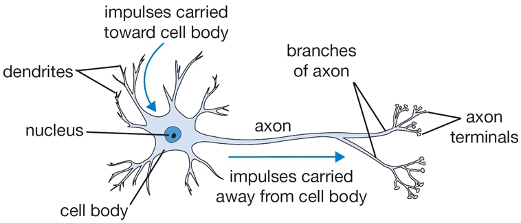
神经科学界的共识是,人脑包含1000亿个神经元,每个神经元有1万个突触,数量巨大,组合方式复杂,联系广泛。也就是说,突触传递机制十分复杂。
现在已经发现和阐明的突触传递机制有:突触后兴奋、突触后抑制、突触前抑制、突触前兴奋,以及远程抑制等。
ANN人工神经网络是一种模仿生物神经网络结构和功能的数学模型,它使用大量的人工神经元连接来进行计算,该网络由大量的“神经元”相互连接构成,每个“神经元”代表一种特定的输出函数。又称激励函数。每两个“神经元”间的连接代表一个通过该连接信号的加权值,称之为权重,这相当于人工神经网络的记忆。网络的输出则根据网络的连接规则来确定,输出因权重值和激励函数的不同而不同。人工神经网络可以理解为对自然界某种算法或者函数的逼近。
下面是一种模拟上述生物神经元的感知器模型。图片来自于Andrej Karpathy在斯坦福课程CS231n上的讲座。
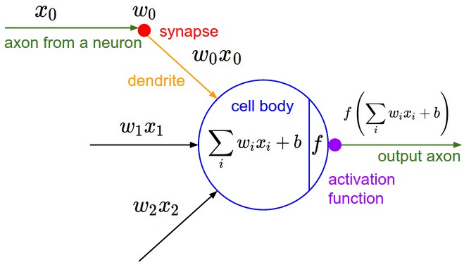
我们可以看到每个神经元或者感知器执行一个带有输入和它的权重的点积,用它们加上偏差,然后应用非线性 $f(x)$,在这种情况下是sigmoid。这个非线性函数也被称为激活函数。
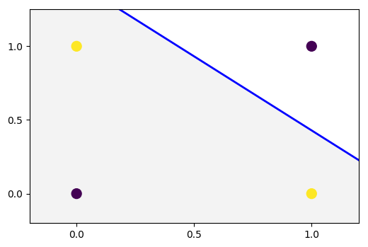
就上图而言,总输入是 $x = x_1 + x_2 + \ldots + x_N$,其中 $N$ 是输入的总数。类别预测取决于特定样本的激活是否导致 $f(z)$ 的输出大于预定阈值。该阈值包含在公式 $z = w_1 x_1 + w_2 x_2 + b$ 中,正如我们在上图中看到的那样,阈值 $b$ 又被称为偏差。为了使它更普遍,有时用 $w_0$ 代替,乘以一个对应的 $x_0$ 得到最终的样子 $z = w_0 x_0 + w_1 x_1 + w_2 x_2$。从图形上看,它看起来像下图,我们在数据中有两个特征 $x_1$ 和 $x_2$。

对于更高维的数据,分界线将是一个超平面。
Rosenblatt感知机是由没过计算机科学家F.Rosenblatt于1957年提出的。F.Rosenblatt经过证明得出结论,如果两类模式是线性可分的,则算法一定收敛。Rosenblatt感知器特别适用于简单的模式分类问题,也可用于基于模式分类的学习控制。
4.3. 单层感知机求解AND/OR问题
原始解法
1 | import matplotlib.pyplot as plt |
结果如下1
2
3W:[ 2.6949501 2.69091272]
b:[-4.2682209]
plot_y: [ 1.78646111 0.38436049]

除了这种每次迭代中逐一处理每个样本的方法,我们可以对公式进行矢量化以减少额外的for循环,使程序运行得更快。下面给出等价的更加简单的实现。矢量化编程在机器学习中非常有用。
1 | import numpy as np |
要特别注意deltaW和deltaB,我们直接将输入x转进行转置,然后乘以误差项。这用到了一个简单的线性代数技巧。最简单的方法就是考虑矩阵大小,输入x是 $4\times 2$ 的,err是 $4\times 1$ 的,那么weights必须是 $2\times 1$ 的。为了得到 $2\times 1$ 矩阵,这里我们直接取了 $x^T\cdot (y-\hat y)$。对于deltaB我们直接求和,得到所有样本点的误差。程序运行求得结果与之前非常接近
1 | W:[ 2.68957829 2.68957829] |

利用TensorFlow求解single-perceptron
现在,让我们使用tensorflow实现相同的感知器算法,看看利用TensorFlow来解决问题的基本流程。在面对海量数据的时候,TensorFlow将会是一个强大的工具。
在TensorFlow中,除了直接定义x和y以外,我们还需要在一个session下定义x和y对应的placeholder,而Variable被申明为TensorFlow中的变量,我们需要在程序运行过程中训练它。TensorFlow函数Variable()有一个名为trainable=True的默认值参数。默认为True时会将其放入计算图进行计算。这里起初并没有更改原先的W和B,而是利用了临时变量W_和B_,将每次迭代更新后得到的参数存储,然后再将它们的值assign到原始的变量W和B中。
完整的程序代码如下:1
2
3
4
5
6
7
8
9
10
11
12
13
14
15
16
17
18
19
20
21
22
23
24
25
26
27
28
29
30
31
32
33
34
35
36
37
38
39
40
41
42
43
44
45
46
47
48
49
50
51
52
53
54
55import numpy as np
import matplotlib.pyplot as plt
import tensorflow as tf
NUM_FEATURES = 2
NUM_ITER = 2000
learning_rate = 0.01
x = np.array([[0, 0], [1, 0], [1, 1], [0, 1]], np.float32) # 4x2, input
y = np.array([0, 0, 1, 0], np.float32) # 4, correct output, AND operation
# y = np.array([0, 1, 1, 1], np.float32) # OR operation
y = np.reshape(y, [4, 1]) # convert to 4x1
X = tf.placeholder(tf.float32, shape=[4, 2])
Y = tf.placeholder(tf.float32, shape=[4, 1])
W = tf.Variable(tf.zeros([NUM_FEATURES, 1]), tf.float32)
B = tf.Variable(tf.zeros([1, 1]), tf.float32)
yHat = tf.sigmoid(tf.add(tf.matmul(X, W), B)) # 4x1
err = Y - yHat
deltaW = tf.matmul(tf.transpose(X), err) # have to be 2x1
deltaB = tf.reduce_sum(err, 0) # 4, have to 1x1. sum all the biases? yes
W_ = W + learning_rate * deltaW
B_ = B + learning_rate * deltaB
# to update the values of weights and biases.
step = tf.group(W.assign(W_), B.assign(B_))
sess = tf.Session()
init = tf.global_variables_initializer()
sess.run(init)
for k in range(NUM_ITER):
sess.run([step], feed_dict={X: x, Y: y})
W = np.squeeze(sess.run(W))
b = np.squeeze(sess.run(B))
# Now plot the fitted line. We need only two points to plot the line
plot_x = np.array([np.min(x[:, 0] - 0.2), np.max(x[:, 1] + 0.2)])
plot_y = - 1 / W[1] * (W[0] * plot_x + b)
plot_y = np.reshape(plot_y, [2, -1])
plot_y = np.squeeze(plot_y)
print('W: ' + str(W))
print('b: ' + str(b))
print('plot_y: ' + str(plot_y))
plt.scatter(x[:, 0], x[:, 1], c=y, s=100, cmap='viridis')
plt.plot(plot_x, plot_y, color='k', linewidth=2)
plt.xlim([-0.2, 1.2])
plt.ylim([-0.2, 1.25])
plt.show()
程序运行结果如下1
2
3W: [ 2.68957829 2.68957829]
b: -4.264309883117676
plot_y: [ 1.78549385 0.38549384]

从上图可以看到,单层感知机模型对于逻辑与/或问题,给出了很好的结果。
多层感知机求解XOR问题
下面我们从一个例子开始介绍多层感知机模型(multi-layer perceptron)。同样,多层感知机是一种监督学习方法。在面临XOR问题时,我们发现single-layer perceptron不起作用了!为了学习XOR问题的特征,我们需要一个至少两层的神经网络,因为XOR问题不能由简单一条直线进行区分。下面我们简单实现一个两层的神经网络来学习XOR模型。对于MNIST手写数字集,我们也可以用类似的多层感知机来进行分类。
对于如下逻辑门

将输入A和B记为x,输出记为y,异或问题在x中元素一致时取0,否则取1。
对于为什么需要两层神经网络有一个直观的理解,如下图
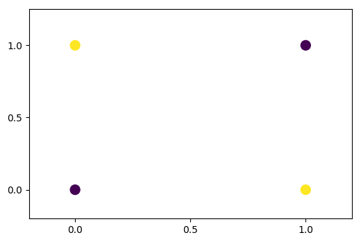
黄点为0,红点为1,那么我们需要两条线来将0和1划分。我们已经看到,神经元/感知器只给我们一条线,将输入空间分成两类。所以我们至少需要在我们第一个隐藏层中的两个神经元来学习异或。我们需要将这两个神经元并排放置在一个层中,而不是放在两个不同的层中,以便他们同时看到输入并学习如何分离输入空间。
下面实现以下最简单的两层神经网络来学习异或门。

Remark:
值得注意的是,一个MLP可以包含任意数量的层和任意数量的神经元。这些通常被称作是超参数(hyperparameters)。如何选择超参数是一个算法设计问题,由实际问题的大小和难度来决定。例如,XOR是一个具有两个特征并且输入大小仅为4的玩具问题。因此,第一个隐藏层中具有2个单位的双层MLP就能够学习XOR函数。一个比较大的问题,例如对mnist数据集中的数字进行分类,将需要在每个layer中使用更多的神经元,后面有机会会讲到。
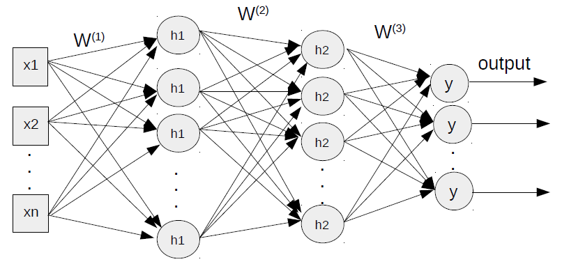
MLP模型确立
我们在单层感知器中已经看到输出是通过将输入x乘以权重w,加上偏差b并最终采用一个非线性sigmoid函数f来激活计算的。
如上图,我们有一个输入层,一个隐藏层和一个输出层,w中的上标表示图层编号。
多层感知器有时被称为普通神经网络(vanilla neural networks),特别是当它们只有一个隐藏层时。
有趣的是,人工神经网络(ANN)的基本结构与单层感知器相似。我们将在所有层中进行相同的计算。
最初我们将我们的输入传到第一个隐藏层,然后第一层的输出被输入到第二层。也就是说,每次我们将当前层的输出视为下一层的输入并执行类似的计算。
隐藏层输出可以通过如下表示
$$
h = g(W^{(1)} x + b^{(1)})
$$
其中,$x$ 为inputs, $g$ 为一个non-linear的激活函数,$W^{(1)}$ 是第一层上的weights,$b$ 是bias。将隐藏层看做输入层,我们可以得到MLP最终层的输出
$$
\hat y = f(W^{(2)} h + b^{(2)})
$$
结合以上两个式子(这个过程称为feed-forward)可得
$$
\hat y = f(W^{(2)} g(W^{(1)} x + b^{(1)}) + b^{(2)})
$$
实际上,无论MLP中有多少图层,数学表达式都是单个方程,其中考虑了从输入开始的所有隐藏层。
简言之,每个多层感知器基于训练数据集学都了某个函数,并且能够将相似的输入序列映射到适当的输出。
Remark:
- 在任何层中,由于权重 $W$ 用于将输入传递到输出,所以它被定义为前后神经元层数的矩阵。例如,在我们的MLP中,$W^{(1)}$是2×2,$W^{(2)}$是2×1。
- 非线性 $g$ 在神经网络中起着重要作用。最常见的非线性类型包括sigmoid,tanh,relu等,以及它们各自的优点和局限性。nonlinear也称为激活函数。
- feed-forward图解

python实现多层感知机求解异或问题
不要忘记导入必要的包含和其他全局变量,如学习速率,迭代次数等等,重要的是要注意最小尺寸的MLP(2个输入,2个隐藏的神经元,1个输出神经元),正如我们在这里实现的,学习XOR可能会很棘手。
可能需要调整learning rate。太大的值(如0.1)是不常用,因为会使网络振荡overshoot。非常低的值(如0.0001)将导致网络学习非常缓慢,可能需要迭代数十万次。
1 | x = np.array([[0, 0], [0, 1], [1, 0], [1, 1]], np.float32) |
下面实现两层感知器模型的辅助函数multi_layer_perceptron_xor。我们使用S型非线性作为激活函数。也可以用其他非线性的函数例如tanh。
Remark:
观察显示tanh比sigmoid具有更高的收敛概率,但这里还是sigmoid。
1 | def multi_layer_perceptron_xor(x, weights, biases): |
权重值的初始化对学习XOR也很重要。我们从一个随机正态分布中选择权重,其均值为0.0,标准差为1.0,并将weights的数据类型设成python字典。
Remark:
- sigmoid和tanh都有一个输出饱和的巨大区域。这些区域的梯度非常小,这在神经网络中不是好的性质。一般我们希望我们的权重在原点周围足够小,以使激活函数在其线性区域中运行,这部分梯度最大。
- 有时候随机初始化可能会遇到一种参数组合,该情形下很容易陷入局部最小值,并且网络不会学到任何东西。所以你在调整参数以减少迭代次数的时候,可能会遇到网络出现两条随机线而不是XOR的解决方案的情况。
1 | weights = { |
创建模型:1
model = multi_layer_perceptron_xor(X, weights, biases)
现在我们需要训练模型。为此,我们定义了一个损失函数和优化器optimizer。由于这是一个二元分类问题,因此使用sigmoid交叉熵损失而不是softmax。
MLP利用一种称为反向传播(因为我们已有标签y)的监督学习方法进行训练。反向传播是任何人工神经网络设计的核心。简而言之,它是通过计算成本函数(cost function)的梯度来调整神经元权重的一种方法。它从输出层开始,并将错误传播回第一层,以便神经元以减少前一次迭代的误差的方式来调整权重。通过这种方式,整个网络最终以一组权重值来较好的解释训练集。
反向传播是一个很大的话题,涉及大量的数学,值得在这方面发表一篇完整的文章。
TensorFlow在这里为我们完成所有这些后台计算,包括梯度,反向传播和权重更新的工作。在这里,我们只需要关注MLP如何工作。
1 | loss_func = tf.reduce_sum(tf.nn.sigmoid_cross_entropy_with_logits(logits=model, labels=Y)) |
用最初设置的迭代次数进行迭代。确保你用足够的迭代训练模型。XOR通常需要大量迭代才能收敛,推荐至少100,000次迭代。你可以使用不同的迭代次数来观察网络的行为。
1 | for k in range(num_iter): |
通过output层,可以绘制出如下的拟合线
完整代码如下1
2
3
4
5
6
7
8
9
10
11
12
13
14
15
16
17
18
19
20
21
22
23
24
25
26
27
28
29
30
31
32
33
34
35
36
37
38
39
40
41
42
43
44
45
46
47
48
49
50
51
52
53
54
55
56
57
58
59
60
61
62
63
64
65
66
67
68
69
70
71
72
73
74
75
76
77
78
79
80
81
82
83
84
85
86
87import numpy as np
import tensorflow as tf
import matplotlib.pyplot as plt
num_features = 2
num_iter = 10000
display_step = int(num_iter / 10)
learning_rate = 0.01
num_input = 2 # units in the input layer 28x28 images
num_hidden1 = 2 # units in the first hidden layer
num_output = 1 # units in the output, only one output 0 or 1
#%% mlp function
def multi_layer_perceptron_xor(x, weights, biases):
hidden_layer1 = tf.add(tf.matmul(x, weights['w_h1']), biases['b_h1'])
hidden_layer1 = tf.nn.sigmoid(hidden_layer1)
out_layer = tf.add(tf.matmul(hidden_layer1, weights['w_out']), biases['b_out'])
return out_layer
#%%
x = np.array([[0, 0], [0, 1], [1, 0], [1, 1]], np.float32) # 4x2, input
y = np.array([0, 1, 1, 0], np.float32) # 4, correct output, AND operation
y = np.reshape(y, [4,1]) # convert to 4x1
# trainum_inputg data and labels
X = tf.placeholder('float', [None, num_input]) # training data
Y = tf.placeholder('float', [None, num_output]) # labels
# weights and biases
weights = {
'w_h1' : tf.Variable(tf.random_normal([num_input, num_hidden1])), # w1, from input layer to hidden layer 1
'w_out': tf.Variable(tf.random_normal([num_hidden1, num_output])) # w2, from hidden layer 1 to output layer
}
biases = {
'b_h1' : tf.Variable(tf.zeros([num_hidden1])),
'b_out': tf.Variable(tf.zeros([num_output]))
}
model = multi_layer_perceptron_xor(X, weights, biases)
'''
- cost function and optimization
- sigmoid cross entropy -- single output
- softmax cross entropy -- multiple output, normalized
'''
loss_func = tf.reduce_sum(tf.nn.sigmoid_cross_entropy_with_logits(logits=model, labels=Y))
optimizer = tf.train.GradientDescentOptimizer(learning_rate=learning_rate).minimize(loss_func)
sess = tf.Session()
init = tf.global_variables_initializer()
sess.run(init)
for k in range(num_iter):
tmp_cost, _ = sess.run([loss_func, optimizer], feed_dict={X: x, Y: y})
if k % display_step == 0:
#print('output: ', sess.run(model, feed_dict={X:x}))
print('loss= ' + "{:.5f}".format(tmp_cost))
# separates the input space
W = np.squeeze(sess.run(weights['w_h1'])) # 2x2
b = np.squeeze(sess.run(biases['b_h1'])) # 2,
sess.close()
#%%
# Now plot the fitted line. We need only two points to plot the line
plot_x = np.array([np.min(x[:, 0] - 0.2), np.max(x[:, 1]+0.2)])
plot_y = -1 / W[1, 0] * (W[0, 0] * plot_x + b[0])
plot_y = np.reshape(plot_y, [2, -1])
plot_y = np.squeeze(plot_y)
plot_y2 = -1 / W[1, 1] * (W[0, 1] * plot_x + b[1])
plot_y2 = np.reshape(plot_y2, [2, -1])
plot_y2 = np.squeeze(plot_y2)
plt.scatter(x[:, 0], x[:, 1], c=y, s=100, cmap='viridis')
plt.plot(plot_x, plot_y, color='k', linewidth=2) # line 1
plt.plot(plot_x, plot_y2, color='k', linewidth=2) # line 2
plt.xlim([-0.2, 1.2]); plt.ylim([-0.2, 1.25]);
#plt.text(0.425, 1.05, 'XOR', fontsize=14)
plt.xticks([0.0, 0.5, 1.0]); plt.yticks([0.0, 0.5, 1.0])
plt.show()
背后细节:
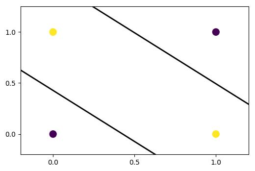
我们已经看到了一个学习XOR的MLP模型。问题是,这个网络是怎样训练出两条可以很好地区分两种输入类型的线?让我们解码一个mlp的内幕。
遵照我们上面建立的XOR网络,我们可以解剖每个神经元的输出,如下面的逻辑表。这里有趣的一点是可以看到第一个隐藏层单元h1和h2学到了什么。
| x1 | x2 | h1 | h2 | y |
|---|---|---|---|---|
| 0 | 0 | 0 | 1 | 0 |
| 0 | 1 | 1 | 1 | 1 |
| 1 | 0 | 1 | 1 | 1 |
| 1 | 1 | 1 | 0 | 0 |
在下面的图中,暗区显示1,而亮区意味着0。第一隐藏单元h1学习权重,以便如下图(红色超平面)所示,它将输入序列中x1和x2均为0的输入与其余的分开。
h2以同样的方式分隔输入,如图蓝色超平面。
这种方式网络提出了以下两种中间解决方案。

你会发现每个h1和h2实际上都是作为单层感知器工作的,其中每个单元实际上都学习了一个单独的线(或超平面)。
Remark:
你也可以把h1当作OR门,把h2当作NAND门。
再观察上面的逻辑表,这两个中间输出将作为输出神经元y的输入。输出单元在其两个输入(h1和h2)为1时响应1,否则保持沉默(或在生物学术语中不反应)。输出y组合了两个超平面,最后我们找到下面的图,它和我们已经看到的xor输出相同。其中,暗区指示1,亮区指示0。

4.4. 利用多层感知机训练MNIST数据集
上面,我们了一个简单的两层MLP来求解XOR问题。为了看到mlp的实际潜力,我们应该设计一个具有两层以上的适度更大的MLP并且看看它在真实世界数据集上是如何工作的。
我们选择mnist作为数据集来实现我们的mlp。尽管mnist被认为是机器学习社区中非常简单的数据集之一,但我们仍然选择这个数据集,因为这将使我们清楚地了解多层感知器的工作原理,并有助于使我们做好使用其他大数据集的准备。后面,我们还可以用mnist数据集来做其他一些很酷的事情,比如使用一些降维技术将每个图像视为2D空间中的一个点。让我们来谈谈关于mnist数据集的一些问题,因为我们在机器学习研究中经常遇到这些数据。
MNIST是手写数字的数据库,由Yann Lecun,Corinna Cortes和Christopher.J.C. Burges创建。有大约60000次训练和10000个测试图像/示例。它是一个名为NIST的更大集合的子集。这些数字已经进行了尺寸标准化并以固定尺寸的图像为中心。图像是 $28\times 28$ 尺寸大小的。作为一个测试平台,我们可以在MNIST数据集上尝试各种学习算法和模式识别方法,同时保持很低的预处理和格式化方面的开销,这使得MNIST成为机器学习中使用最广泛的数据集之一。我们不必担心自己下载数据集,只需要TensorFlow里的一条命令tensorflow.examples.tutorials.mnist就可以获取。
1 | from tensorflow.examples.tutorials.mnist import input_data |
首先,我们来看几个样例:

图像是 $28\times 28$ 大小的并且随机的。训练数据由 $55,000$ 个样本组成,因此大小是 $55000\times 784$。训练的labels是 $55000\times 10$ 大小的(10是类别数量0到9)而不是 $55000\times 1$。这是因为它们采用one-hot向量的格式,其中只有相应的位置标签为1,其余为零。例如,如果训练样本是2,则相应的单热矢量将是[0,0,1,0,0,0,0,0,0,0]。
下图是MNIST样本在2d空间中的快照。
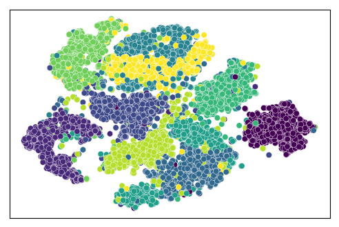
我们看到10个集群,分别对应10位数字。一些集群相互交织在一起,这是因为有些数字看起来很相似。例如,数字“4”和数字“9”在手写中有时看起来相似。所以很可能这两个数字在像素空间中彼此靠近。
可视化是在将维数从784减少到2(使用t-SNE)之后创建的。后面有机会会讲一些维数降低技术。
MLP模型:
以下是我们要实施的mlp。我们有784个输入像素,用x表示,128个h1神经元,256个h2神经元和10个y或输出神经元。
我们在单层感知器中已经看到,输出 $\hat y$ 是通过将输入 $x$ 乘以权重 $W$,加上偏差 $b$ 并最终采用非线性sigmoid函数 $f$ 来计算的。这里我们有一个输入层,两个隐藏层和一个输出层,如上图所示,$W$ 中的上标依旧表示网络层数编号。
ANN的基本构件与单层感知器相似。我们将在所有层中进行相同的计算。最初我们有我们的输入到第一个隐藏层,然后第一个隐藏层的输出被输入到第二个隐藏层。
每次我们将当前输出视为下一层的输入并执行类似的计算。隐藏层输出公式如下
$$
h1 = g(W^{(1)} x + b^{(1)})
$$
现在隐藏层输出h1将作为第二隐藏层h2的输入,并且h2层的输出作为输入到输出层y的输入。
$$
h2 = g(W^{(2)} h1 + b^{(2)})
$$
结合上式,有
$$
h2 = g(W^{(2)} g(W^{(1)} x + b(1)) + b^{(2)})
$$
得最后的输出
$$
\hat y = f(W^{(3)} h2 + b^{(3)})
$$
这里没有将它们全部结合起来,用x,h1和h2表示y。因为看起来会很杂乱。实际上,我们在前面已经说过,无论MLP中有多少图层,数学表达式都可以是输出的单个方程,其中包括了从输入开始的所有隐藏层。简言之,每个多层感知器基于训练数据集学习单个函数 $f(\cdot)$,并且能够将相似的输入序列映射到适当的输出。
Remark:
依然作为附注,在任何层中,由于权重W用于将输入传递到输出,所以它通常被定义为前后神经元层数之间的矩阵。例如,在我们的mlp中,W1是784x128,W2是128x256,W3是256x10。
多层神经网络:
MLP能做的不只是学习一个简单的异或门。基于以上,我们可以非常轻松地插入新layer来完成更苛刻的分类。让我们再添加一层到目前为止实现的层。
在XOR中,我们在输出层只有一个神经元,输出0或1。MNIST是一个数字的数据库,所以现在我们有10个输出神经元表示从0到9。
假设我们在第一个隐藏层中有128个神经元,第二个中有256个神经元。
现在我们有10个输出神经元,输入是784维,它们是图像的每个像素。
我们在每次迭代中一次处理100个图像,这就是为什么我们将批量大小设置为100(可以是小于图像总数的任何其他数字)。
1 | batch_size = 100 |
以下我们定义神经网络的辅助函数。使用我们在上一篇文章中看到的相同的数学表达式,我们定义了1层,2层等等。你可以看到在另一个层增加一层很容易。这里我们在输出层之前添加了隐藏层2。
1 | def multi_layer_perceptron_mnist(x, weights, biases): |
对于我们的三层MLP,我们定义每个层的权重和偏差为python字典。
1 | weights = { |
注意,在这里我们使用了一个不同的损失函数,softmax带logits的交叉熵,我们用来学习异或操作的东西是sigmoid。原因是这个数据集有两个以上的类。S形交叉熵损失仅用于二元分类问题。
1 | loss_func = tf.reduce_mean(tf.nn.softmax_cross_entropy_with_logits(logits=model, labels=y)) |
您可能会注意到,不是使用梯度下降作为优化器,而是使用adam作为优化器。adam代表自适应动量估计。它是随机梯度下降算法的替代方法之一,它自己为每个参数自适应地更新学习速率。adam是类似adagrad,adadelta,rmsprop等其他优化算法的升级,它计算每个参数的自适应学习速率。除了存储过去平方梯度的指数衰减平均值之外,它还保持与动量相似的过去梯度的指数衰减平均值。
现在训练模型进行一些迭代。一起处理55000个图像,这被称为批处理,在计算的上下文中是低效的。另一方面,逐一处理每个图像,这被称为随机处理,也有不利的一面。由于每个梯度都是基于单个训练样例进行计算的,因此误差比噪声梯度下降更大。在这两个极端情况下,我们提出了一种小批量技术,我们在这里称之为batch_size,在此处处理一大块图像。小批量学习可以理解为将批量梯度下降应用于训练数据的较小子集,例如一次100个样本。与批量梯度下降相比,优势在于通过小批量更快地达到收敛,因为更频繁的权重更新。没有关于将多少图像用作批量大小的定义规则。
正如我们在上一篇文章中提到的,MLP利用监督式学习(因为我们提供了标签)技术,称为反向传播训练。反向传播是任何人工神经网络设计的核心。简而言之,它是通过计算成本函数的梯度来调整神经元权重的一种方法。它从输出层开始,并将错误传播回第一层,以便神经元以减少前一次迭代错误的方式调整权重。通过这种方式,整个网络以一组权重值来确定训练集(希望测试集也是如此)。tensorflow强在幕后处理所有这些梯度计算,反向传播和权重更新。
1 | for iter in range(num_iter): |
随着迭代的进行,您将看到损失函数在下降,如下图所示。左图显示损失按照迭代进行下降,并在某个点几乎达到饱和。在右侧,准确度从大约90%开始。最初准确性急剧增加,这基本上是损失函数大幅下降的原因。在某个点上,准确度也会在一个很小的范围内得到修正。


我们看到我们的MLP在找到10位数类的非线性分类方面做得非常好。准确度在95.45%左右。每次运行情况可能会有所不同。你可以改变不同层次的单元/神经元的数量,批量大小等,并查看网络的行为。
完整代码如下:1
2
3
4
5
6
7
8
9
10
11
12
13
14
15
16
17
18
19
20
21
22
23
24
25
26
27
28
29
30
31
32
33
34
35
36
37
38
39
40
41
42
43
44
45
46
47
48
49
50
51
52
53
54
55
56
57
58
59
60
61
62
63
64
65
66
67
68
69
70
71
72
73
74
75
76
77
78
79
80
81
82
83
84
85
86
87
88
89
90
91
92
93
94
95
96
97
98
99
100
101
102
103
104
105
106
107
108
109
110
111
112
113
114
115
116import tensorflow as tf
import numpy as np
import matplotlib.pyplot as plt
# %% data
# read mnist data. If the data is there, it will not download again.
from tensorflow.examples.tutorials.mnist import input_data
mnist = input_data.read_data_sets('/path/to/MNIST/', one_hot=True)
# look at some of the images. randomly
rand_img = np.array([2500, 1001, 100, 500])
for i in range(np.size(rand_img, 0)):
plt.subplot(1, 4, i+1)
plt.axis('off')
plt.imshow(np.reshape(mnist.train.images[rand_img[i]], [28, 28]), cmap='gray')
print('Training data size : ', mnist.train.images.shape)
print('Training label size: ', mnist.train.labels.shape) # labels are in one-hot vector
# print(mnist.train.labels[rand_img])
# %% create the MLP model
def multi_layer_perceptron_mnist(x, weights, biases):
"""
MLP model with more than 2 hidden layers.
"""
hidden_layer1 = tf.add(tf.matmul(x, weights['w_h1']), biases['b_h1'])
hidden_layer1 = tf.nn.relu(hidden_layer1) # apply ReLU non-linearity
hidden_layer2 = tf.add(tf.matmul(hidden_layer1, weights['w_h2']), biases['b_h2'])
hidden_layer2 = tf.nn.relu(hidden_layer2)
out_layer = tf.add(tf.matmul(hidden_layer2, weights['w_out']), biases['b_out']) # NO non-linearity in the output layer
return out_layer
# %% construct the MLP model
# hyper-parameters
learning_rate = 0.01
num_iter = 30
batch_size = 100
display_step = 10 # display the avg cost after this number of epochs
# variables
num_input = 784 # units in the input layer 28x28 images
num_hidden1 = 128 # units in the first hidden layer
num_hidden2 = 256
num_output = 10 # units in the output layer 0 to 9. OR nClasses
# trainum_inputg data and labels
x = tf.placeholder('float', [None, num_input]) # training data
y = tf.placeholder('float', [None, num_output]) # labels
# weights and biases
weights = {
'w_h1': tf.Variable(tf.random_normal([num_input, num_hidden1])), # w1, from input layer to hidden layer 1
'w_h2': tf.Variable(tf.random_normal([num_hidden1, num_hidden2])), # w2, from hidden layer 1 to hidden layer 2
'w_out': tf.Variable(tf.random_normal([num_hidden2, num_output])) # w3, from hidden layer 2 to output layer
}
biases = {
'b_h1': tf.Variable(tf.random_normal([num_hidden1])), # b1, to hidden layer 1 units
'b_h2': tf.Variable(tf.random_normal([num_hidden2])),
'b_out': tf.Variable(tf.random_normal([num_output]))
}
# construct the model
model = multi_layer_perceptron_mnist(x, weights, biases)
# cost function and optimization
loss_func = tf.reduce_mean(tf.nn.softmax_cross_entropy_with_logits(logits=model, labels=y))
optimizer = tf.train.AdamOptimizer(learning_rate=learning_rate).minimize(loss_func)
# %% Train and test
sess = tf.Session()
init = tf.global_variables_initializer()
sess.run(init)
cost_all = np.array([])
acc_all = np.array([])
# Train the model
for iter in range(num_iter):
avg_cost = 0.0
num_batch = int(mnist.train.num_examples / batch_size) # total number of batches
for nB in range(num_batch):
trainData, trainLabels = mnist.train.next_batch(batch_size=batch_size)
tmp_cost, _ = sess.run([loss_func, optimizer], feed_dict={x: trainData, y: trainLabels})
avg_cost = avg_cost + tmp_cost / num_batch
correct_pred = tf.equal(tf.arg_max(model, 1), tf.arg_max(y, 1))
accuracy = tf.reduce_mean(tf.cast(correct_pred, 'float'))
acc = accuracy.eval(session=sess, feed_dict={x: mnist.test.images, y: mnist.test.labels})
if iter % display_step == 0:
print('Epoch: %04d' % (iter+1), 'cost= ' + "{:.5f}".format(avg_cost), 'accuracy: ' + "{:.5f}".format(acc))
cost_all = np.append(cost_all, avg_cost)
acc_all = np.append(acc_all, acc)
print('Optimization done...')
# plot the accuracy and loss
x_data = range(num_iter)
plt.plot(x_data, cost_all, color='r')
plt.xticks([0, 10, 20, 30])
plt.yticks([0, 10, 20, 30, 40])
plt.show()
plt.plot(x_data, acc_all)
plt.xticks([0, 10, 20, 30])
plt.yticks([0.9, 0.95, 1.0])
plt.show()
今天内容就止步于此,相信关于感知机大家还有很多问题,比如就刚才这个问题,对3层MLP的简单扩展将会增加一层,看看它是否会改变网络的结果。从理论上讲,如果将这4层MLP应用于MNIST数据,分类准确性应该更高,至少略高一点。不过事实情况建议大家自己尝试。
5. Exercise:
- 用简单神经网络训练逻辑与的运算,尝试不同的学习率
1 | inputs = np.array([[1, 1], [1, 0], [0, 0], [0, 1]]) |
将一组 $(x, y)$ 值划分为下面两类函数之一
- $2x+1=y$ 为第1类
- $7x+1=y$ 为第2类
训练数据
1
2inputs = np.array([[1, 3], [2, 3], [1, 8], [2, 15], [3, 7], [4, 29]])
labels = np.array([1, 1, -1, -1, 1, -1])由函数定义可知,$[9, 19]$ 属于第1类,$[9, 64]$ 属于第2类。
1
29 19 => 1
9 64 => -1输出训练之后的神经网络权值参数,最后用 $[9, 19]$ 和 $[3, 22]$ 对训练成功的网络进行测试
- 验证如下数据集上,Rosenblatt感知机算法的局限性
1 | inputs = np.array([[1, 1, 6], [1, 3, 12], [1, 3, 9], [1, 3, 21], [1, 2, 16], [1, 3, 15]]) |
Hint:


